2.1

The Rate Equations Model

The light-matter interactions occurring in a SL can be modeled in a simple way by using the RE model [1, 4]. The RE model considers the interplay between carriers and photons in the laser cavity in terms of conservation equations. The number of electrons and holes is assumed to be the same, thus only one equation for carriers is considered in the model. The main assumption of the model is that carriers and photons are considered to be uniformly distributed in the longitudinal and transversal directions.

Assuming a single mode laser, the relationship between the carrier density, N(t), the photon density, S(t), and the optical phase, ϕ (t), can be expressed by the following equations:

where the descriptions of the symbols and their values are given in Tab. 1. Typical values for a 1550 nm Distributed Feed Back (DFB) laser [5] are used by default.

Table 1.

Symbols and default values used in Eqs. 1-3.

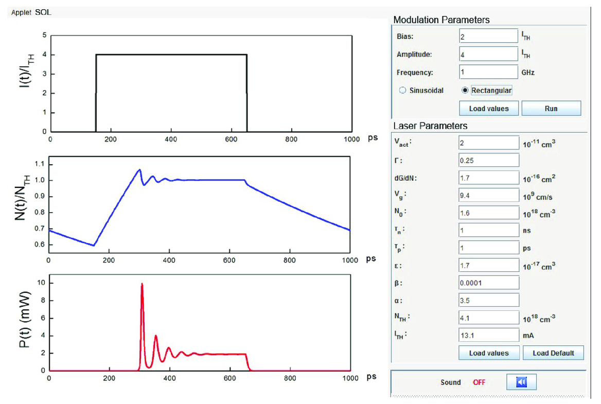
The RE model previously described has been implemented in Java® [6] programming language and the resulting applet is hosted by Universidad Politécnica de Madrid, in a web server at Tecnología Fotónica y Bioingeniería (www.tfo.upm.es/educational-tools). Equations 1-3 are solved with a Runge Kutta iterative algorithm for N(t), S(t) and ϕ(t), with temporal resolution of 1 ps for a vector of 10000 points (10 ns).

2.2

The Graphic User Interface

The Graphic User Interface (GUI) is shown in Fig. 1. It is composed of four panels and three graphs. From the Modulation Parameters panel the user can choose the current waveform, the bias point, the peak-to-peak amplitude and the frequency of the modulating current. The waveform of the current can be selected by the user, either sinusoidal or rectangular.

Figure 1.

The Graphic Unit Interface.

The laser parameters can be introduced by the user in the Laser Parameters panel, placed on the right side of the GUI. Values shown in Tab. 1 are considered by default. Carrier density threshold (N_TH) and threshold current (I_TH) are calculated as N_TH = N₀ + (τ_P·dG/dN·v_GΓ)^-1 and I_TH = N_TH·q·V_act·τ_N^-1, by solving Eqs. 1-2 in steady state regime at threshold.

By pressing the Run button in the Modulation Parameter panel, the program solves Eqs. 1-3, and returns the values of carrier density, photon density and optical phase at each temporal instant. The instantaneous frequency, v(t), is calculated from the temporal derivative of the phase, as v(t) = (2π)^-1d/dt(ϕ(t)). Three graphs on the left side of the GUI show the results of the simulation. From up to down, the temporal profiles of injected current, carrier density and output power are shown. Current and carrier density are plotted as a function of I_TH and N_TH, respectively.

From the laser intensity and chirp, the software builds an amplitude and frequency modulated signal of the form A(t)·cos(2π(f₀ + f(t)), where A(t) is proportional to S(t), f(t) is the frequency v(t) shifted into the audible frequency range. This conversion is obtained with a constant factor of 10⁹, changing nanoseconds into seconds and GHz into Hz. The Sound control is placed at the bottom of the right side of the GUI and allows switching on and off the reproduced sound. The Save Data panel allows the user to export the simulation results to a text file, where the time, current, number of carriers, output power and instantaneous frequency vectors are stored in a tab separated format.

3.1

Laser Switch On

We first consider the simple case in which the SL is switched on with a rectangular current function. In order to have this, in the Modulation Parameters panel, the rectangular current waveform is selected, I_BIAS is set to 1.5 I_TH, the amplitude is set to 3 I_TH and the frequency is set to 0.25 GHz (4 ns period with 50 % duty cycle).

This corresponds to inject the laser with a current step function with low level equal to 0 and a high level current of 3 I_TH. The laser parameters are set to the default values.

After the Run button is pressed, the program takes some seconds to complete the simulation and the results are finally shown in the GUI graphs. Current, carrier density, output power and instantaneous frequency are exported with the Save Data button and results are plotted in Fig. 2 (a) and (b).

Figure 2.

Results obtained with the rectangular current waveform selected, bias set to 0 and amplitude 3 ITH: (a) current and carrier density, black line left axis and blue line right axis, respectively and (b) output power and chirp, red line left axis and blue line right axis, respectively. The time axis is zoomed 3 ns around the laser switch on.

When the rectangular current is applied, the carrier density grows as 1- exp(-t/τ_N) from the low level steady state to N_TH, as expected from theory [1, 4]. N(t) undergoes damped oscillations around the threshold density value before reaching the steady state value clamped at N_TH. This corresponds to the relaxation oscillations of the output power, due to carrier induced gain modulation, and of the instantaneous frequency, due to the carrier induced index modulation.

The user can appreciate in an intuitive manner, the coupled amplitude/frequency modulation, by pressing the Sound in the GUI. As expected, when the laser is off, for I(t) = 0, no sound is produced, then a chirped sound is emitted, when power and instantaneous frequency oscillate, and finally a single frequency tone is produced, corresponding to the optical carrier of the laser shifted into the audible band.

3.2

Direct Modulation

In this example, we consider the direct modulation of the laser with a periodic rectangular current waveform, with the low and high current level both above the threshold current value I_TH. In the Modulation Parameters panel, the rect current waveform is selected, BIAS is set to 4 I_TH, the amplitude is set to 2 I_TH and the frequency field is set to 0.5 GHz. After pressing the Run button, the results are plotted in the GUI graphs. In this case, the well known phenomenon of transient and adiabatic chirp in DM SLs is clearly appreciated after listening to the audible output. The transient chirp is usually referred to the instantaneous frequency variation associated to the transition between the two levels of the injected current, i. e. the damped oscillations of v(t) which follows from low to high and from high to low current level transitions. The adiabatic chirp is the frequency difference between the frequency produced during the high level and the frequency produced during the low level of injected current. The adiabatic chirp is directly related to the gain compression factor ε. As shown in Fig. 3 (a) and (b), the carrier density is not clamped to the threshold value NTH as in the ideal case (ε = 0).

Figure 3.

Results obtained with the rectangular current waveform selected, bias set to 4 I_TH, amplitude 2 I_TH and frequency 0.5 GHz: (a) current and carrier density, black line left axis and blue line right axis, respectively and (b) output power and chirp, red line left axis and blue line right axis, respectively.

In the proposed simulation, the audio output is composite of a single higher tone during the high level state, a lower single tone during the low level state (corresponding to the adiabatic chirp) and a chirped sound when the current switches from low to high level and viceversa (corresponding to the transient chirp). This is also appreciated from the instantaneous frequency temporal profile, where the frequency difference between low and high level of the injected current due to the adiabatic chirp, is clearly shown in Fig. 4 (a) and (b). If the gain compression factor ε is set to zero, the adiabatic chirp signature disappears from the audio output and the graphs, as expected from theory.