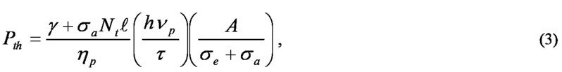
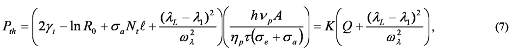
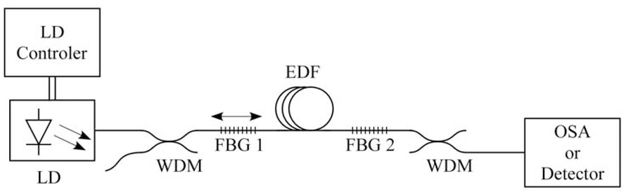
1.1

Introduction

The use of erbium doped fiber amplifiers (EDFA’s)^{1, 2} has been established as a corner stone in today’s optical communication networks either in long distance/high bit rate links or in local networks. Fiber laser market is growing due to its many advantages over conventional lasers^{2, 3}. Among others it should be pointed the advantage of fiber lasers in the Aerospace sector due to its inherent lightweight, robustness and low maintenance, and in the Industrial sector by the flexibility of fiber light guiding and delivery, allowing its integration within industrial robots. From the above considerations it is clear that laboratory activities with fiber amplifiers and lasers are a must in a Photonics Laboratory. Excellent laboratorial activities for exploring the EDFA behavior have been reported^{4, 5}, including the development of some laser systems.

This experiment was implemented for a first year master’s degree laboratory class for Physical Engineering students from the Physics and Astronomy Department at the University of Porto (http://dfa.fc.up.pt). Each weekly class had four hours duration. During the same semester the students attended classes on lasers, semiconductors and applications and magnetic materials and applications. Despite the fact that this communication only reflects the results of the implementation of a fiber laser, students had prior contact with fiber processing techniques (such as cleaving and splicing), spectroscopic characterization (of absorption and fluorescence phenomena) and studied an optical fiber amplifier assembled with the same fiber used in this experiment: the amplifier study followed the procedures presented in the works of Johnstone et al⁴ and Zhu et al⁵. The laser was usually assembled and tested in a single class.

Our approach to fiber lasers is based on a Fabry-Perot cavity built with two fiber Bragg gratings (FBG)^{6, 7} with a small mismatch in the Bragg wavelength. The laser emission is achieved when this mismatch is reduced through longitudinal stress applied to one of the gratings. This approach is very interesting since it permits students to gain sensitivity to the lasers characteristics as a function of the cavity parameters, in particular mirror reflectivity (total losses) in what concerns both threshold and slope efficiency. Complementary the use of FBGs as guided optical sensors can also be introduced in a transversal way. In this work typical optical sensing structures, namely the FBGs, are used in an inverse way to control the laser cavity parameters.

A Bragg grating is a periodic perturbation of the refractive index along the waveguide, and is formed by exposing it to an intense ultraviolet periodic light pattern created by the interference of two light beams at the same wavelength.

A very common method to fabricate Bragg gratings is based on a diffractive optical element, and is usually referred as the phase mask method, Figure 1. The phase mask consists of a high quality fused silica plate (transparent at the writing wavelength) that contains a one dimensional surface relief structure on its surface. A UV beam incident on the phase mask is thus diffracted by the surface relief grating, and the depth of the grooves of the mask dictates the power distribution among the diffraction orders. The depth value is chosen in such way that the zero order diffracted beam is minimized (typically to less than 5%), while the ±1 diffracted orders are maximized. A spatially modulated UV field is obtained by the interference of these two first order beams, and the period of the pattern is one half of the period of the phase mask relief grating.

Figure 1.

Schematic illustration of the phase mask technique for Bragg grating photo-inscription

To fabricate Bragg gratings it is essential that the waveguide materials, within the core media are photosensitive, i.e., that its refractive index can be permanently changed through UV exposure. Usually, this property can be found in optical fibers doped with germanium. In some cases, such as the ones where the germanium doping is low, photosensitivity enhancement through molecular hydrogen in-diffusion has to be performed.

The refractive index perturbation usually consists of a core geometry variation and/or of a core index perturbation, both inducing an effective index perturbation. The resulting uniform sinusoidal Bragg index grating along the core of the waveguide can be expressed as:

where n₀ is the average index, Δn is the UV induced refractive index perturbation, z is the distance along the longitudinal axis and Λ is the spatial period of the index modulation. For this periodic modulation the central Bragg resonant wavelength is given by:

where n_ff is the effective index of the propagating mode. Therefore, the Bragg wavelength can be changed by varying the period, such as by stretching or compressing the fiber, or by affecting the modal effective index such as by temperature change.

1.2

Theory

Our discussion starts from the theory presented in Orazio Svelto book⁸, chapter four, the same bibliography the students use for the lasers course.

The pump laser threshold (P_th) for a quasi-three-level laser is given by⁸:

where, h is the Planck constant, σ_a and σ_e are respectively the absorption and emission cross-sections, N_t, is the number of active atoms per volume unit, ℓ is the length of the active medium, η_p is the pump laser efficiency, ν_p is the frequency of the pump laser, τ is the upper level lifetime, A is the section of the active medium and γ is the single pass logarithmic loss.

The total logarithmic loss per pass arises from the intrinsic loss (γ_i) and from the losses induced by the two mirrors (y₁ = −ln(R₁) and γ₂ = −ln(R₂)), and is obtained from:

Assuming that both gratings are identical in reflectivity, with central Gaussian profile,

where R₀ is the maximum reflectivity and ω_λ is the 1/e half width, we get

As laser emission occurs at the wavelength where losses are minimum, it can be easily shown that the laser emission will take place at λ_L = (λ₁+λ₂)/2 if both gratings overlap. As (λ_L-λ₁)² = (λX_L-λ₂)², using equations 4 and 6 in equation 3 it can be written as:

showing a quadratic behavior of the laser threshold pump power with grating shift.

The laser efficiency (η_s), defined as the slope of the laser output power versus pump power, above threshold, is given by⁸:

where ν_L is the laser emission frequency and A_b is de laser mode area inside de fiber.

Using equations 4 and 6, this equation can be rewritten as:

By using this equation with prior knowledge on R₀ and ω_λ from the FBG characterization, one can obtain λ_i and an estimation of η_p.

3.1

Fiber Bragg grating characterization

The fluorescence due to the erbium doped fiber can be easily measured with the OSA, when the cavity is detuned, i.e different Bragg peaks for each FBG. The spectrum measured by the OSA at the near end of the cavity is shown in Figure 4. Some structure is seen around 1540 nm, from which the working characteristics of FBG’s can be clearly observed and discussed with the students: the positive peak is due to spontaneous emission light being reflected by FBG1 in the far end at its Bragg wavelength, and the negative peak is made by the reflectivity of FBG2 in the near end.

Figure 4.

Fluorescence spectra from the fiber laser (inset linear scale), showing the effect of the two fiber Bragg gratings.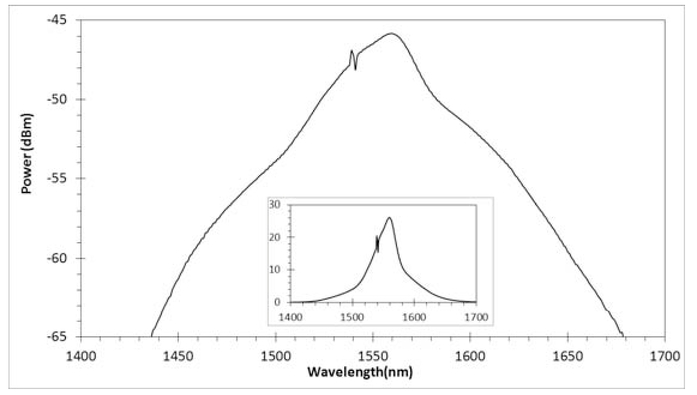

By changing the FBG1 stretching conditions, its Bragg wavelength is changed, thus moving the positive peak location – see Figure 5. Again, the positive peaks are due to spontaneous emission reflected by FBG1 in the far end, and the negative peaks are made by the reflectivity of FBG2 in the near end. For a certain position, between 7.35 and 7.45 mm, both FBGs are tuned to the same Bragg wavelength, thus the cavity retains the spectral energy around that Bragg wavelength for both FBGs are reflecting the same spectral region.

Figure 5.

Spectra from the fiber laser, below threshold, for different stage positions (in millimeters). The positive peaks are due to spontaneous emission reflected by FBG1 in the far end, and the negative peaks are made by the reflectivity of FBG2 in the near end.

Noting that due to the way the fiber was glued onto the stretching translation stage, an increase in the position corresponds do a decrease in fiber length, as expected, in Figure 5 the FBG1 shows a shift to higher wavelengths as it is stretched. A linear fit of the maximum wavelength vs position gives a sensitivity of −7.797 nm/mm and a crossing of the two peaks at 7.4133 mm.

From the analysis of the spectral attenuation around the Bragg wavelength of FBG2, the grating reflectivity can be reconstructed as a function of wavelength. The results presented in Figure 6 were obtained by measuring the attenuation of the negative peak against wavelength around the FBG2 Bragg wavelength. Then, the reflectivity function can be reconstructed from:

Figure 6.

FBG2 reflectivity. From the fitting we obtain a maximum reflectivity of 75.8% and a width of 0.111 nm (1/e half width).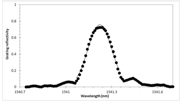

where Δdbm(λ) is the attenuation relative to the original fluorescence spectrum.

3.2

Laser characterization

Spectral emission characteristics

Fiber laser operation should be characterized in terms of laser emission content as a function of the optical pump power increase. For this study, the FBG1 is stretched until a good overlap with FBG2 is obtained. Then the laser spectrum is recorded for increasing values of pump power. Figure 7 shows different spectra obtained between 4 and 33 mW pump power on the proposed experimental configuration. The spectrum in curve A was obtained below threshold and shows a behavior similar to the ones presented in Figure 5. Just below threshold, curve B, a small increase in output power is clearly visible, and in curve C this peak grows to a 35 dB peak with a small increase in pump power. The 3 dB width of the laser peak was measures to be 0.07 nm. Finally, curve D shows the spectrum well above threshold obtained with 33 mW of pump power. At these conditions a rise to ∼40 dB signal to noise ratio can be measured, preserving the width measured in curve C.

Figure 7.

Spectra for different pump powers: A- 4 mW, B- 5 mW, C- 6 mW and D- 33 mW.

Laser power & Laser threshold characteristics

To study the dependence of laser output power as a function of pump power, the OSA is replaced by an optical power meter, and the laser output power should be measured for a set of pump power, and for different stretching’s of FBG1 thus creating different wavelength mismatch. Results obtained for the described setup are presented in Figure 8. For each set, a linear fit was performed along the output power linear behavior section, in order to obtain the threshold pump power value and the slope efficiency. Figure 8 shows three representative curves, clearly showing that the threshold increases with the decrease of reflectivity, and that the best efficiency is not obtained with the lower cavity losses (triangular data point marker). These results were obtained using the power measured after FBG2, at the near end output. Considering that both outputs have similar output power, the maximum estimated output efficiency of this non optimized laser is around 20% (twice the value obtained from fig 8).

Figure 8.

Output power as a function of pump power for different stage positions. Triangles 7.410 mm (Δλ = −0.0155 nm), circles 7.435 mm (Δλ = 0.0819 nm), squares 7.440 mm (Δλ = 0.1014 nm).

As introduced by equation 7, the laser threshold pump power is expected to have a quadratic dependency with the grating detuning. In Figure 9 laser pump power threshold is plotted as a function of absolute position in the translation stage (proportional to the wavelength detuning, as suggested by equation 2). A parabolic fit was performed with its minimum fixed to the position corresponding to tuned gratings (7.4133 mm) showing a good agreement with the experimental values.

Figure 9.

Threshold pump power vs stage position. The quadratic fit assumes the minimum at the position where the two gratings overlap (7.4133 mm).

Laser efficiency

In Figure 10 the inverse of the slope efficiency is plotted against the wavelength difference between laser emission and the peak reflectivity of the two gratings. Using the values of −ln R₀ = 0.277 and ω_λ = 0.1106 nm, obtained from the FBG reflectivity characteristics, we obtained from the fit γ_i = 0.15 and, assuming that the mode area is about the same as the doping area, we can estimate η_p as ∼38%.

Figure 10.

Inverse of the slope efficiency vs wavelength shift from the grating peak reflectivity to laser wavelength. Fitting to equation 9 using the measured grating reflectivity and width as fixed parameters.