2.1.

Elementary objects

The file dioptre.m in the directory @dioptre contains the definition of the classe named dioptre. It is used for implementing refracting interfaces which are characterised by their location on the optical axes, their radius of curvature and the refractive indexes of the two media. Likewise, the file mirror.m in the directory @mirror contains the definition of the classe named mirror. It is used for implementing reflecting interfaces which are characterised by their location on the optical axes, their radius of curvature and the refractive index of the media. Finally, the file diaphragm.m in the directory @diaphragm contains the definition of the classe named diaphragm.

The functions defined in the private directories perform elementary actions on the corresponding optical subsystem like setting some characteristics, returning the transfer matrix R or the propagation one T, computing the intersection of a ray with the interface, …

2.2.

Transfer matrix

When considering complex optical system consisting of regions of free space with a constant refractive index separated by spherical refracting/reflecting surfaces between the input and the output front planes, Exy and Sxy, the optical system is homogeneous step by step. Propagation through this system can be treated with the elementary matrices R and T corresponding to the refraction/reflection at an interface and to the propagation through free space [1]. The product of these elementary matrices, written from right to left following the path of the light, is the transfer matrix of the optical system within the GAUSS approximation:

The function matrix returns in the variable T the transfer matrix T_ES of the optical system between the input plane Exy and the output plane Sxy:

The vector soc contains the individual elements of the optical system. Since the first cell of soc is used for storing the positions of the input and output planes Exy and Sxy as well as the refractive indexes n_o and n_i of the initial and final media, T is initialized with the transfer matrix of the first element reached by the light, here stored in the second cell. Then, products with propagation and transfer matrices are used up to the last element to obtain the final transfer matrix between Exy and Sxy.

The function power returns the opposite of T(2,2) which is by definition the refractive power V of the optical system.

2.3.

Cardinal elements

The function focal returns in the two variables fo and fi the object and image focal lengths f_o = −n_o/V and f_i = n_i/V:

where No and Ni are the refractive indexes n_o and n_i of the initial and final media, and V is the power V of the optical system as returned by the power function.

The function cardinal returns in the six variables EFo, SFi, EHo, SHi, ENo and SNi the location of the focal planes ( and ), the principal planes ( and ) and the nodal points ( and ) with respect to the input and output planes Exy and Sxy:

where T is the transfer matrix T_ES of the optical system returned by the matrix function.

2.4.

Algebraic determination of an image point within Gauss approximation

The function homographic returns in the variable SAi the position of an image A_i:

where EAo is the position of the object A_o. The function invhomographic performs the reverse operation:

These two functions also return in the three variables Gt, Ga and Gl the transversal, angular and longitudinal magnifications G_t, G_a and G_l:

where TaoAi is the transfer matrix between the conjugate planes A_oxy and A_ixy:

and is easily derived from the transfer matrix T_ES of the optical system and the transfer matrices describing the propagation between the front planes A_oxy and Exy on one hand, Sxy and A_ixy on the other hand.

The function descartes returns in the variable HiAi the position of an image A_i computed with the aid of Descartes’s relation with regards to the principal points:

where H0A0 is the position of the object A_a. The function invdescartes performs the reverse operation:

In addition, these functions also return the three magnifications:

Finally, the newton function returns in the variable FiAi the position of an image A_i computed with the aid of Newton’s relation with regards to the focal points:

where F0A0 is the position of the object A_o. The function invnewton performs the reverse operation:

In addition, these functions also return the three magnifications:

or

2.5.

Graphical determination of an image point within Gauss approximation

The function plotcardinal plots the position of the cardinal elements on an optical axis where the input and output planes Exy ans Sxy of the optical system are also drawn.

For a given object A_oB_o at a distance from Exy and for the corresponding image A_iB_i located at a distance from Sxy, the function plotgaussrays plots the three particular rays:

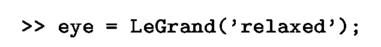
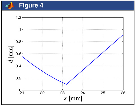
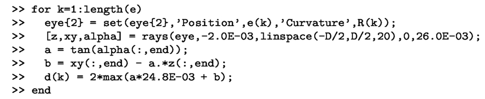
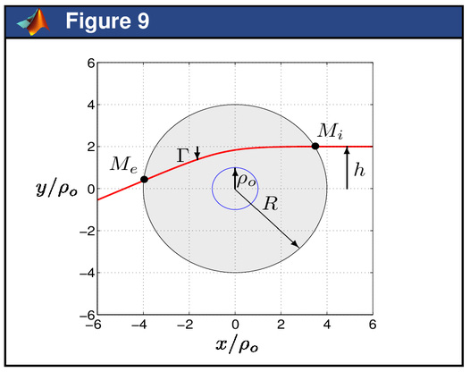
2.6.

Ray tracing

When propagating within the optical system, the rays are refracted/reflected by the successive interfaces. Between these interfaces, light is travelling in straight line in an homogeneous media. The corresponding rays are characterized by a set of coordinates (z, xy) (namely the coordinates of the intersection point with each interface) and by an inclination angle a with the optical axis which are computed with the aid of Snell-Dedcartes laws. The function rays returns in the variables z, xy and a the successive locations and inclinations of these rays:

The function ray is a private function of the elementary classes described in section 2.1 which propagates the ray though each individual element of the optical system soc. The function rays is ended by computing the propagation of the ray after the optical system up to a plane, namely a virtual screen. Finally, the path of the rays can be plotted with the function plotrays.

3.1.

Gauss approximation

The transfer matrix is easily obtained with the matrix function:

Then the focal distances are returned by the focal function:

Finally, the cardinal elements are computed with the cardinal function:

and they represented in Fig. 1 with the plotcardinal function:

Figure 1

The total power of the eye is returned by the power function:

It can be checked that approximately two third of this power is due to the cornea:

The optical distance e between the cornea and the lens can therefore be computed with the aid of Gull-Strand’s formula. Indeed, since the refractive index of the aqueous, the medium between the posterior face of the cornea and the anterior face of the lens, is 1.3374, we have:

It can be verified that e is equal to the distance between the image principal plane of the cornea and the object principal plane of the lens by computing the cardinal elements of these two optical subsystems. The iris is the aperture stop of the eye. The position EP_e of input pupil P_e with respect to the input plane Exy can be obtained with the aid of the invhomographic function:

since it is the conjugate point of the aperture stop given by the optical elements in front of the latter (i.e. here the cornea). It is located 3.04 mm behind Exy, that is to say 0.56 mm in front of the iris. Taking into account the transversal magnification, its diameter is equal to 6.78 mm. Likewise, the location of the output pupil P_s with respect to the output plane Sxy is obtained with the aid of the homographic function:

since it is the image of the aperture stop given by the optical elements behind the latter (i.e. here the lens). It is located 3.92 mm in front of the output plane Sxy, that is to say only 0.08 mm behind the iris. Accounting for the transversal magnification, its diameter is equal to 6.25 mm.

3.2.

Ray tracing and aberrations

We now consider an incident beam of 20 rays parallel to the optical axis. The diameter of this beam is, for example, 6 mm, and the path of the rays will be plotted from a plane located 2 mm in front of the cornea to another plane 26 mm behind it in the vicinity of the retina:

The result is represented on Fig. 2 with the aid of the plotsysopt and plotrays functions:

Figure 2

It can be observed that the eye is not an optical system which can be only studied within the Gauss approximation. For example, the localization of the retina, that is to say the localization of the image focal plane, requires a ray tracing procedure. From the final coordinates and inclination of the rays when they hit the plane located 26 mm in the back of the cornea, the equation of the rays emerging from the lens can be computed:

Then, the distance z = −b/a from the origin where the rays cross the optical axis is computed:

The variations of the radius of the incident beam r wrt. z are shown on Fig. 3:

Figure 3

This figure illustrates the fact that incident rays parallel to the optical axis are all the more convergent when they are far from the optical axis. Moreover, all the rays cross the optical axis before the image focal plane whose location in the Gauss approximation is 24.2 mm from the anterior face of the cornea. Finally, the diameter d of the spot in a plane located at a given distance z from the anterior face of the cornea can be computed:

The variations of d wrt. z are shown on Fig. 4:

Figure 4

It can be observed that the smallest spot, whose diameter d is here about 0.1 mm, is not in the focal plane but in a plane which is 1 mm in front of it:

since it is located 23.2 mm behind the anterior face of the cornea compared to 24.2 mm in the GAUSS approximation.

The following figures show that the localization of the retina is not a matter of GAUSS approximation but requires a ray tracing procedure since it is always over-estimated by the former approach.

3.3.

LASIK

Nowadays, some ametropias of the eye (myopia and hypermetropia) could be corrected by means of a modification of the shape of the anterior face of the cornea. A photo-ablation of a small piece of the cornea is obtained with the aid of an excimer laser. After cicatrizing, the radius of curvature of the anterior face of the cornea is modified. The refractive power of the cornea is changed accordingly, and the ametropic eye becomes emmetropic. This surgical technique is knows under the acronym LASIK which stands for Laser ASsisted In-situ Keratomileusis. One of the problems encountered in practice is to evaluate the amount of cornea removal in order to give to the cornea the expected refractive power [6]. We show in this section that a ray tracing approach could be very helpful to achieve this goal since it is the only way to properly take into account aberrations of the cornea [7].

The free parameters for the photo-ablation of a piece of cornea are the thickness ε of the corneal tissue which is burned as well as the diameter D of the surgical field. The goal is to change the radius of curvature R of the anterior face of the cornea so that, after cicatrizing, the new radius of curvature R′ leads to a better focussing of the rays on the retina. Both radii are related to each other with the following equation [1]:

Measurements of keratometry and pachymetry of an eye suffering from myopia have led to the following numbers:

The diameter of the surgical field D has been fixed to 6 mm. The radius of curvature of the reshaped anterior face of the cornea R′ is here computed for different values of the thickness ε:

The variations of R′ wrt. ε are represented on Fig. 5:

Figure 5

Measurements have shown that the retina is located 17.2 mm behind the posterior face of the lens, that is to say 24.8 mm behind the anterior face of the cornea. The diameter d of the spot on the retina is computed for an incident beam of 20 rays parallel to the optical axis. The width of this beam is taken equal to D:

The variations of d wrt. ε are represented on Fig. 6:

Figure 6

The thickness of the tissue to be burned corresponds to the value of ε for which d is minimal:

These values can be compared to those before correction, namely those for ε = 0:

The thickness of the corneal tissue to be burned is ε = 77 μm in the simulated surgical conditions. The diameter of the spot in the retina plane is therefore reduced from d = 0.78 mm down to less than d = 0.09 mm. To reach this goal, the radius of curvature of the anterior face of the cornea has increased from R = 7.25 mm up to R′ = 8.14 mm.

The consequence of this change of the radius of curvature is illustrated in Figs. 7 and 8 where the path of rays are plotted before and after corneal tissue removal:

Figure 7

Figure 8

Paying attention to the path of the rays close to the retina plane located 24.8 mm behind the anterior face of the cornea, it is observed that after correction the rays are converging on the retina whereas they were converging before the retina plane before correction since the eye was suffering from myopia.

The same simulation can be conducted with different values for the diameter D of the surgical field. The corresponding numbers show that, like expected, the thickness ε of the corneal tissue to be burned for reaching the same goal is an increasing function of D.