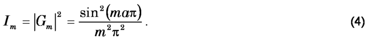
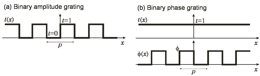
1.

INTRODUCTION

Diffraction is a topic usually introduced in general physics courses and taught more extensively in more advanced optics courses in Physics and Engineering degrees. Diffraction gratings have been regarded as one of the most important instruments in physics¹ and they are indeed an important educational tool for describing the wave nature of light. Usually, in general physics textbooks^2-4, they are analyzed on the basis of a direct application of the Huygens principle. The angular directions where the diffraction orders are generated are easily derived from the condition of constructive interference between the wavelets transmitted through the multiple slits of the diffraction grating.

However, as it is noted in some general physics textbooks², this simplified approach does not explain the relative intensities of the diffracted orders nor the grating’s angular resolving power, because the envelope associated with the slit width is ignored. The effect of this envelope function is so important that some diffraction orders may disappear, although they fulfil the former interference condition. For instance, the simplest binary amplitude diffraction grating, where the width of the slit is half the period of the grating, produces a diffraction pattern where all even diffraction orders are missing. A full quantitative analysis of diffraction gratings is usually taught in advanced optics courses based on the Fourier transform description of the multislit interference phenomena, characteristic of the Fraunhofer approximation⁵. However, the use of Fourier theory to analyze diffraction problems is too advanced for introductory physics courses.

In this work we show a simpler method to fully describe binary diffraction grating patterns. The analysis is based on a phasor technique directly derived from the Huygens principle, where we take into account the phase contributions from all points at the slit aperture. The addition of all these contributions results in a slit phasor, whose length is directly related to the diffraction order amplitude. The contribution of all the slits leads to the so-called grating phasor which describes the grating’s resolving power. We study binary amplitude diffraction gratings with different fill factors (ratio between the transparent and opaque areas). When changing the grating’s fill factor the relative intensities of the different diffraction orders are modified, and the missing orders change.

While diffraction gratings are usually introduced considering amplitude gratings, phase-only diffraction gratings are much more attractive for technological purposes because of their much greater diffraction efficiency. Additionally, the recent advent of liquid crystal technology allows the realization of programmable phase-only gratings⁶. In this work we also show how to extend the proposed phasor analysis to binary phase-only diffraction gratings. Within this intuitive formalism, the grating’s diffraction efficiency, which is an important quality parameter of a diffraction grating and is assimilated to the intensity of the positive first diffraction order, can be easily obtained. The proposed phasor analysis of diffraction gratings explains such properties in a physically very intuitive way, and provides an interesting teaching tool for undergraduate students in general physics courses, where diffraction is not studied on the basis of the Fourier transform.

A similar phasor analysis is considered in some fundamental physics textbooks in order to address specific diffraction problems. For instance, it is used to analyze the diffraction pattern of a single slit^2,4. In other texts^3,7, it is applied to multislit interference and it describes the increasing intensity and narrowing of the main peaks as the number of slits increases. However, to our knowledge, no general physics textbook shows the connection between the phasor analysis and the Fourier transform calculation. This connection is not shown, either, in more advanced optics books⁵, where diffraction gratings are directly treated on the Fourier transform basis. In this work we demonstrate that the diffraction’s order amplitude calculated within our slit phasor formalism is mathematically equivalent to the one obtained by the Fourier transform calculation.

Finally, the proposed phasor analysis is illustrated experimentally in the case of binary amplitude diffraction gratings by using a ferroelectric liquid crystal display, which allows to very easily change the diffraction grating’s fill factor simply by changing the addressed image. The experiment agrees very well with the theory, and it is an illustrative optical demonstration.

2.

PHASOR ANALYSIS OF BINARY DIFFRACTION GRATINGS

We consider diffraction gratings illuminated with plane wave monochromatic light with normal incidence and wavelength λ. The grating’s period is regarded to be high enough so that the scalar diffraction theory is valid, and we concentrate on describing the diffraction pattern generated in the Fraunhofer approximation.

For simplicity we start considering binary amplitude gratings as described in Fig. 1(a). The period p is divided in two regions, with transmittances t₁=1 and t₂=0 and widths d₁ and d₂, respectively. The gratings period is constant p=d₁+d₂, but we consider different relative widths of the two regions. A fill factor parameter a can be defined such that d₁=ap and d₂=(1-a)p. The grating has N slits and its extension is A=Np. Figure 1(b) shows the typical diagram used in introductory physics to explain the generation of the diffracted orders by these amplitude diffraction gratings². The angular directions associated to the diffraction orders are obtained from the constructive interference of the Huygens wavelets generated at each aperture. This condition requires that, for the angular direction θ_m where the m diffraction order is generated, the path difference between the waves generated at the same point at consecutive apertures must be equal to an integer number of wavelengths, mλ. Therefore, for instance, points A and A’ in Fig. 1(b) are in phase. This situation, leads to the very well-known diffraction grating law^2,3:

Fig. 1.

(a) Diffraction grating transmittance g(x) of a binary amplitude diffraction grating with period p, fill factor a=d₁/p and width A=Np, being N the number of slits. (b) Ray diagram at the diffraction grating plane, where θm is the angular direction of the m diffracted order.

However, the above condition does not explain the relative intensities of the different diffraction orders, in particular the vanishing of some orders.

2.1

The slit phasor: relative intensity of diffracted orders of binary amplitude gratings

Based on the Huygens principle, an intuitive phasor analysis which explains not only the angular direction of the diffraction orders but also their relative intensities, can be developed. The idea of this method is based on considering the phase mismatch of all the wavelets scattered in the diffraction order angular direction from all points in the slit aperture, and is illustrated in Figure 1(b). We consider the phase mismatch of the rays emerging from the slit aperture with diffraction angle θ_m at all points in the wavefront between A and C. Each contribution can be represented by a phasor in the complex plane whose orientation is given by the phase state of the corresponding wavelet. The amplitude of the corresponding diffraction order is given by the magnitude of the phasor resulting from adding all these contributions. We call this phasor the slit phasor since it is directly related to the slit’s shape. Figure 2 shows the slit phasor diagrams for the zero (undiffracted) and the first four diffraction orders (see figure columns) of binary gratings with different fill factors (see figure rows).

Fig. 2.

Slit phasor diagrams for diffraction orders m=0, 1, 2, 3, 4, and for fill factors a=1/2, 1/3 and 1/4.

Let us first consider the simplest binary amplitude diffraction grating, where the period is divided in two equal regions with transmittances 1 and zero (fill factor a=1/2). For the zero diffraction order, there is not a phase difference between the transmitted rays, and all the phasors are aligned, being the total length equal to 1/2, corresponding to the mean half-intensity transmission in a single period. For the first order (m=1), the difference in path lengths between rays A and B is λ/4, and between ray A and ray C is λ/2 (Fig. 1(b)). Consequently, the phase at point A is zero, while the ray crossing at point B contributes with a phase π/2, and the ray crossing at point C contributes with phase π. Therefore, these rays are represented in Figure 2 by a phasor parallel to the positive real axis (ray A), parallel to the positive imaginary axis (ray B) and parallel to the negative real axis (ray C). The summation of all the phasors contained between A and C results in a total phasor along the positive imaginary axis, whose square modulus gives the intensity of the diffraction order m=1 for the diffraction grating with fill factor a=1/2.

Let us now consider the diffraction order m=2. Now, ray A’ in Fig. 1(b) contributes to the wavefront with a phase 4π, (the path from the grating is 2λ). Rays A, B and C follow paths 0, λ/2 and λ, and therefore they contribute with phases 0, π and 2π respectively. Then, the phasor contributions fill the whole complex plane and the total summation is cancelled. This explains why the second diffraction order has zero intensity. For m=3, the phasors related to rays A, B and C have phases 0, 3π/2 and 3π. Therefore, all the phasors contributing to the third diffraction order are contained in one and a half complex plane and the density of phasors is smaller than for m=1, namely, it is one third of that value. Hence, we expect the intensity of the third order I₃ to be one-ninth of I₁. Finally, in the case of m=4, the total phasor contributions fills twice the complex plane and the total summation is cancelled. This is why the fourth diffraction order has zero intensity.

We now consider the diffraction grating with fill factor a=1/3. In the ray diagram of Figure 1(b) the path for ray C is now mλ/3. The corresponding phasor diagrams are shown in the second row of Figure 2. The rays contributing to the first order are those between A and C in Figure 1(b) whose difference in path length is λ/3. Therefore, the contributing phasors have phases from zero to 2π/3 and they result in a non-zero total phasor with squared modulus I₁. For m=2, ray C corresponds to a phasor with phase 4π/3, and the density of phasors is reduced by one half. Hence, the expected relative intensities between the second and first diffraction order is I₂/I₁=1/4. For m=3, the difference in path length between rays A and C in Figure 1(b) is λ, and they correspond to phasors with phases zero and 2π. Therefore, all the contributing phasors are contained in the whole complex plane and their summation is exactly cancelled. This explains why now the third order is missing. For m=4, the phasor distribution is similar to the case m=1, but the phasor density is one fourth. Therefore their intensity ratio is I₄/I₁=1/16.

Finally, we consider the diffraction grating with fill factor a=1/4. For the first diffraction order, only the first quadrant in the complex plane is filled. For diffraction orders 2 and 3 the phasors are distributed in two and three quadrants of the complex plane. In this case, the phasors are distributed along the whole complex plane for the fourth diffraction order, and therefore this is now the vanishing order.

For the correct evaluation of the diffraction orders intensity, it is required to calculate the density of phasors (D) when these are distributed on an angular sector. Since for the zero diffracted order all the slit phasors are aligned, the total phasor length is equal to a. When considering the m^th diffracted order, the phasors are uniformly distributed in an angular sector ma2π, and therefore:

2.2

Connection between phasor and Fourier analysis

Here we demonstrate that the slit phasor analysis above described provides the exact solution of the diffraction orders amplitude derived from the Fourier transform analysis. In our approach, this amplitude is given by the total slit phasor length. In the Fourier transform analysis, this amplitude is given by the diffraction’s grating Fourier expansion coefficient of the corresponding order. A detailed comparison between the phasor and the Fourier transform approach is developed in a previous work⁸. We show below that these quantities have an equivalent mathematical expression. This demonstration is interesting for educational purposes, since it is usually not included in general physics textbooks - because it is too advanced -, nor in more advanced optics books, where diffraction gratings are described only on a Fourier transform basis.

The relative intensities of the diffraction orders are not affected by the grating’s extension provided the number of slits is large. Therefore we can assume an infinitely extended diffraction grating, and use the Fourier expansion series to obtain the value of the Fourier coefficients Gm corresponding to the amplitude of the m^th diffraction order. They can be calculated as⁵:

where the function g(x) describes the grating’s transmittance, being g(x)=1 when x∊[0,ap], and zero in the rest of the period, and where the change of variables θ=m2πx/p, has been applied. Let us note that the second equality in Eq. (3) exactly corresponds to the slit phasor calculation in Section 2.1. The integrand term is the phasor exp(iθ), which is integrated from 0 to the maximum value ma2π. This depends on the diffraction order m and the fill factor a, exactly as the phasors described in section 2. On the other hand, the factor (m2π)^–1 exactly corresponds to the density of phasors mentioned in the previous subsection. The intensity of the diffraction orders is then given by:

The limit m→0 of this expression is equal to a², in agreement with the phasor of length a at m=0.

Therefore, the above discussion demonstrates that the phasor analysis described in Section 2, which was derived from physical considerations, leads to the same expression for the diffraction orders amplitude as the Fourier series analysis. Table I summarizes the intensities of the first diffraction orders for different fill factor values. We can see that all the conclusions previously derived from the slit phasor analysis are confirmed from this exact Fourier calculation.

Table I:

Relative intensities of the first diffraction orders for binary amplitude gratings with different fill factors.

Fill factor	I0	I±1	I±2	I±3	I±4
a=1/2	1/4=25.0%	1/π2=10.1%	0	1/9π2	0
a=1/3	1/9=11.1%	3/4π2=7.6%	3/16π2=1.9%	0	3/64π2=0.5%
a=1/4	1/16=6.2%	1/2π2=5.1%	1/4π2=2.5%	1/18π2=0.6%	0

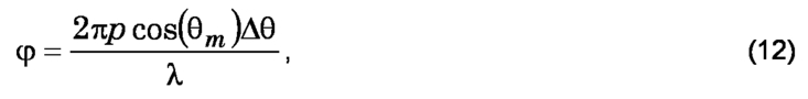
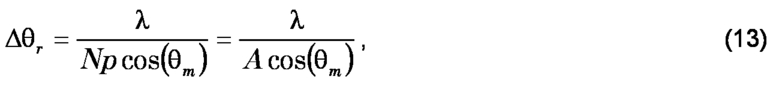
2.3

Extension to binary phase gratings

The phasor analysis can be easily extended to binary phase-only gratings with a relative phase shift ϕ between the two levels in the grating. For the sake of simplicity we consider these levels of equal width (a=1/2). Figure 3 shows the profiles of both the binary amplitude and binary phase grating. The transmittance profile for the latter is g(x)=t(x)exp[iϕ(x)] (t denotes the amplitude and ϕ the phase), which in the centered basic period (x∊[–p/2,+p/2]), is defined as:

Fig. 3.

Transmittance profiles of the binary amplitude and binary phase gratings.

Thus, there are now two different regions in the diffraction grating’s period that contribute to the diffraction pattern, and provide different distributions in the phasor diagrams. The region x∊[0,+p/2] is equivalent to that of an amplitude diffraction grating, whose phasor distribution was analyzed in Fig. 2. But the region x∊[–p/2,0] now contributes with another set of phasors. Figure 4 illustrates the phasor diagrams of the binary phase grating, for the same diffraction orders considered in Fig. 2. The two regions in the grating are distinguished with phasors in two colours, blue for the region with phase ϕ, and red for the area with zero phase.

Fig. 4.

Slit phasor diagrams for diffraction orders m=0,1,2,3,4, of the binary phase grating. Red phasors correspond to the region with zero phase and blue phasors to the region with phase ϕ.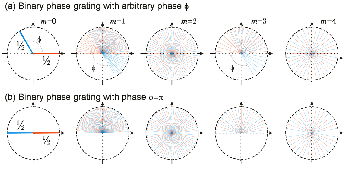

Figures 4(a) and 4(b) illustrate, respectively, the case of arbitrary phase shift ϕ, and the important particular case of ϕ=π radians. Let us first analyze the undiffracted zero order. In this case all the phasors in the same region contribute with the same phase, oriented with phases zero (red phasors) and ϕ (blue phasors). Since the two regions in the grating have the same size (a=1/2), the length of the corresponding phasors is the same (equal to 1/2), and the amplitude of the resulting phasor is the given by

The intensity at this order is therefore I₀=|G₀|²=cos²(ϕ/2). For ϕ=π, the two phasor contributions are aligned in opposite directions and they cancel each other, thus leading to a null intensity.

For the other diffraction orders (m≠0), these phasor contributions are folded according to Eq. (3). Red phasors fold in the positive sense (counterclockwise), while blue phasors fold in the negative sense (clockwise) because they correspond to negative values of x. Since a=1/2, the folding range is the same for the two regions, and increases with m as [0, ±mπ], being the starting angle 0 and ϕ respectively. For m=2, both phasor contributions cover the whole complex circle, resulting in a null global phasor which indicates the zero intensity at this order. This is a consequence of the fact that the two regions in the grating have the same width, and the fill factor is 1/2.

Let us now focus on the odd diffraction orders, and particularly on m=1. Now the phasors cover a wide, but not full, sector of the complex plane. The amplitude of the global phasor can be calculated by applying Eq. (3), which now results in

where, once again, the change of variables θ=m2πx/p, has been applied. Equation (7) shows how the same distribution of phasors of the amplitude grating contribute with two starting angles, 0 and ϕ+π. When ϕ=π the distribution of phasors corresponding to each region exactly overlap, thus producing a multiplicative factor 2 in the resulting total phasor when compared with the amplitude grating (and therefore a multiplicative factor 4 in the intensity). In the case m=3, the linear phases cover a much larger angular sector. In fact, what was covered in an angular sector of π radians for m=1, is now covered in a range of 3π radians. Those phasors covering the angular sector of 2π radians cancel each other, and only the rest contribute to the global phasor. The result is a phasor diagram for m=3 equivalent to that for m=1, but now the density of phasors has been decreased by a factor of 3. The integration in Eq. (7) leads to

The corresponding intensity values are:

Table II gives the intensity values of the first four diffraction orders. The intensity of the positive first diffraction order is the grating’s diffraction efficiency. The phasor analysis of phase diffraction gratings allows to obtain this important quality parameter in a physically intuitive way. As it is expected, we obtain that the diffraction efficiency is maximum for a π-phase grating.

Table II:

Intensity of the first diffraction orders of a binary phase diffraction grating with phase shift ϕ.

3.

THE GRATING PHASOR: RESOLVING POWER

The slit phasor analysis in Section 2.1 deals only with the interference condition of the Huygens wavelets generated by a single slit in the angular direction corresponding to the diffraction order. Now we address the phasor analysis for a different subject: the grating’s angular resolving power. For that purpose we analyze Fig. 5(a), where some rays leaving the grating with a slight angular separation ∆θ from the diffraction order angle have been drawn. We evaluate the phase condition of the Huygens wavelets interference in this angular direction.

Fig. 5.

(a) Ray diagram at the diffraction grating plane for an angular mismatch ∆θ relative to the diffraction order angle θ_m. (b,c,d) Grating phasor diagrams for successive slits n; phasors from successive slits have angular separation φ=2πp∆θ/λ: (b) in the diffraction order angle (∆θ=0), (c) in an angular direction separated ∆θ from the diffraction order angle; (d) in the angular direction where the first zero intensity is obtained.

We consider a non-zero diffraction order angle θ_m. Therefore, the slit phasor associated to each slit in this angular direction is not zero. The key point to derive the angular resolving power is to consider the interference from the multiple slits that constitute the grating. Since the angle ∆θ is very small, we can consider that the slit phasor is approximately still valid also for the angle θ_m+∆θ. Each slit contributes with the slit phasor derived in the previous section. The so called grating phasor is generated by the addition of all the slit phasors oriented in accordance with the interference between the wavelets emerging from the same point of successive slits. As an example we consider points A and A’ in Fig. 5(a). Now the propagation distance from the slit plane (point S) to the point A’ is

The small angle approximation can be applied to ∆θ to obtain that sin(θ_m+∆θ) = sin(θ_m)cos(∆θ)+cos(θ_m)sin(∆θ) ≈ sin(θ_m)+cos(θ_m).∆θ. Taking into account the grating equation (Eq. (1)), the previous equation becomes

Wavelets from successive slits do not interfere exactly in phase, but the phase between them is equal to m2π+2πp·cos(θ_m)·∆θ/λ. We define the angular phasor mismatch as:

This quantity represents the angular separation in the phasor diagram between slit phasors from successive slits. Figure 5(b-d) illustrates the situation, where n labels the slits and N is the total number of slits. Figure 5(b) corresponds to the diffraction order angle θ_m (∆θ=0). In this case all slit phasors from successive slits are always in phase, thus contributing to a grating phasor with a large modulus that explains the diffraction order. When ∆θ≠0 there is a phase mismatch φ between successive slits, given by Eq. (12). The global grating phasor resulting from the addition of all these slit phasors with phase mismatch φ (Fig. 5(c)) has a smaller modulus than the one where ∆θ=0 (Fig. 5(b)), thus explaining the reduction in intensity as ∆θ increases. The first zero intensity angle (which defines the angular resolution ∆θ_r of the grating), is obtained when all the N individual slit phasors are distributed in the whole complex plane, leading to a zero global grating phasor, as shown in Fig. 5(d). This situation is obtained when the condition (N+1)φ=2π, which is simplified to Nφ=2π because the number of slits is in general very large (N>>1). Taking into account this condition and the definition in Eq. (12), the angular resolution is obtained as

This angular separation determines the grating’s resolving power in spectroscopic applications. The smaller ∆θ_r, the greater the resolving power of the grating is.

Two spectral lines with wavelengths λ±∆λ/2 are considered resolved if the maximum of one wavelength coincides with the minimum of the other, i.e. their angular separation is ∆θ_r. The grating’s resolving power (R) is defined^7,9 as R=λ/∆λ. The chromatic dispersion ∆λ is related to the angular resolution ∆θ_r and can be derived from Eq. (1) as

where the small angle approximation has been used again for ∆θ_r. Therefore, considering Eqs. (13) and (14), the resolving power is deduced to be:

This very well known result shows why a larger-size grating has higher resolution, and it has been derived here directly using the grating phasor analysis.

4.

EXPERIMENTAL DEMONSTRATION

The properties described in the previous sections can be easily demonstrated by means of a liquid crystal (LC) microdisplay. LC devices have been used as programmable diffractive screens¹⁰, and also for pedagogical demonstrations⁶. As an example, we will show the change in the vanishing diffraction orders as the fill factor changes. The binary modulation provided by ferroelectric LC displays (FLCD) makes them particularly useful to implement binary diffraction gratings. FLCDs are binary modulators that provide at the output two orthogonal linearly polarized states depending on the addressed voltage¹¹. In this case, the two grating levels are controlled though the standard PC computer video signal.

Here we use a reflective ferroelectric LC on silicon display from CRL-Opto, model RXGA1.5C, with an active area of 12.3 mm × 9.2 mm with 1024×768 pixels. The pixel pitch (distance between pixels) is 12.0 µm × 12.0 µm, being the pixel size 11.4 µm × 11.4 µm (thus the fill factor is about 90%). The FLCD is illuminated with a collimated linearly polarized plane wave of a He-Ne laser, with wavelength λ=632.8 nm. One linear polarizer is placed on the reflected beam, in order to act as an analyzer and operate the FLCD in the binary amplitude modulation scheme. The reflected beam is propagated a distance of about 2 meters in order to observe the diffraction pattern in the Fraunhofer approximation regime. Finally, we use a CCD camera to record the intensity patterns of the diffracted field.

Figure 6 shows the binary images that are addressed to the FLCD and the corresponding experimental diffraction pattern. The three images shown in Fig. 6 are binary amplitude gratings, with fill factor values a=1/2, 1/3 and 1/4, respectively. White pixels refer to areas where the reflected light is transmitted through the analyzer. Black pixels refer to areas where the reflected light is being absorbed by the analyzer. Therefore, the display acts as a binary amplitude diffractive element with transmission values 0 and 1 at the black and white pixels of the addressed image.

Fig. 6.

Diffraction gratings with fill factors a=1/2, 1/3 and 1/4, addressed to the FLCD, with their corresponding experimental diffraction intensity patterns and their profiles.

The experimental diffraction patterns show the typical diffraction orders, and their intensities follow the expected behaviour described in the previous sections. Namely, for the binary grating with fill factor a=1/2 all even orders in the diffraction pattern are cancelled. For the gratings with fill factors a=1/3 and a=1/4, it is the ±3 orders and the ±4 orders the ones that are cancelled, respectively. In these experiments the DC zero order has been slightly over exposed in the CCD camera in order to easily observe the other diffraction orders.

5.

CONCLUSIONS

Using interference considerations on the basis of the Huygens principle, we have developed a phasor technique which provides a complete description of binary diffraction gratings in the Fraunhofer approximation. We have shown how this physically intuitive phasor technique describes, by means of the so called slit phasor, the diffractions amplitude and vanishing orders in the diffraction pattern of binary amplitude gratings with different ratios between the transparent and opaque areas. Also, defining a grating phasor, we have obtained the grating’s resolving power. By applying this formalism to phase-only binary gratings, we have been able to describe the intensity of the diffracted orders and the diffraction efficiency, which is a key quality parameter of the grating.

Such properties of binary amplitude and phase diffraction gratings cannot be addressed in a general physics course, where diffraction gratings are usually explained from the direct application of the Huygens principle. Within this principle only the angular directions of the diffraction orders are described, but not their relative intensities, nor the grating’s angular resolving power and diffraction efficiency. A full description of binary diffraction gratings is usually addressed with the Fourier optics theory in advanced optics courses, which is too complicated for general physics courses.

Thus, in this work we have shown that a simple phasor approach provides a full description of binary diffraction grating patterns in the Fraunhofer approximation. We have also demonstrated that the diffraction’s order amplitude calculated within this phasor formalism is mathematically equivalent to the one obtained by the Fourier transform calculation. The proposed phasor analysis is more intuitive than the Fourier transform approach, and is appropriate for less advanced courses. It also represents an alternative approach to the problem which can be useful for understanding the physical phenomena.

Finally, an illustrative optical demonstration of these effects has been performed by using a ferroelectric liquid crystal display, which allows to very easily change the diffraction grating’s fill factor simply by changing the addressed image.