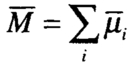
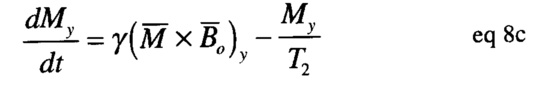
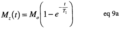
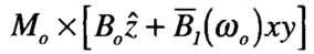
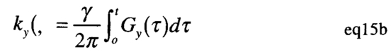
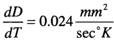
1.1

Nuclear Magnetic Resonance (NMR)

Although NMR is fundamentally a quantum mechanical phenomenon, it is often intuitively described using a mixture of quantum and classical mechanics. This mixed model can be used to describe proton NMR that is primarily involved in magnetic resonance imaging of tissues. If a macroscopic sample of water is placed in a static external magnetic field, it becomes “magnetized”. This magnetization does not happen instantaneously. It requires some characteristic time T₁ to reach an equilibrium-magnetized state. The sources of this magnetization are the magnetic moments of hydrogen protons in the water molecules. This magnetic moment is a fundamental property of the proton. The origin of the proton magnetic moment (μ) can be classically modeled as a current loop with a magnitude equal to the current times the area of the loop (see Fig. 1).

This magnetic moment can be easily related to the angular momentum of the loop by considering a mass, m_p, with charge, e⁺, moving with angular momentum, m_pVr. Thus,

where is the angular momentum, and the direction of is the same as . Next we interject the quantum angular momentum for which we know the magnitude is ; where ℏ is Planck’s constant divided by 2π, and I can only have integer or half integer values. For the proton , therefore the magnitude of . In addition, quantum mechanics tells us that the direction of the quantum angular momentum cannot be known; we can only know the projection of the angular momentum along a given axis. In the case of the proton the projections are . Also, since there are two possible projections for along any given direction, there are two energy states for protons in an external magnetic field.

Needless to say, when we use the known value for proton mass, charge, and angular momentum, the predicted magnitude of the magnetic moment does not agree with measurement. So a correction factor is assigned:

where the g-factor is scaled such that μ agrees with measured values.

This relationship is also written:

with γ being defined as the gyromagnetic ratio, equal to 2.675 × 10⁸ Hz per Tesla for protons.

The interaction of the proton magnetic moment with an external magnetic field, , has energy given by:

and a torque given by:

The first equation (4a) implies a lower energy state exists when the magnetic moment projection is aligned with the direction of the external magnetic field. The second equation implies that magnetic moment will precess around the direction defined by the magnetic field with angular frequency ω_o = γB. This is known as the “Larmor frequency”, which is in the radio frequency (RF) range for imaging applications.

As a two energy state system in thermal equilibrium, the ratio of magnetic moments aligned with the external B-field to moments aligned opposite to the B-field will be less than one from the

The bulk magnetization, over all protons in a unit volume. Therefore in thermal equilibrium:

where N is the number of proton per unit volume.

The equation of motion for in a static field is given by:

which describes a precession of around the direction of with an angular frequency of ω_o = γB. However, in the equilibrium state, will always be aligned with . For the non-equilibrium case the system can be described with three equations that include transient terms that drive the magnetization to the equilibrium-state. These are referred to as the Bloch equations:

where is chosen to be along the z-axis . These equations have solutions of the form:

which for eq. 9a implies that M_z = M_o as t → ∞.

Solutions for eqs 9b,9c are of the form:

The transverse magnetization, M_xy → 0 as t → ∞.

The characteristic times T₁ and T₂ are referred to as the spin-lattice relaxation time constant and the spin-spin relaxation time constant, respectively. The T₁ relaxation involves both conservation of energy and conservation of angular momentum. Therefore, this relaxation has to exchange energy hω_o and angular momentum with the surrounding medium or lattice. Consequently we expect T₁ to have temperature dependence proportional to e^–ε_a/kT. The T₂ relaxation does not require any energy exchange since there is no magnetic field along the x or y axis. Thus, it only requires conservation of angular momentum in units of . This interaction involves fluctuations in the local magnetic field seen by the proton. Such fluctuations are often associated with unpaired magnetic moments such as that found in paramagnetic materials. These fluctuations are temperature dependent as well: ∝ sηe^{–ε / kT} where S is a geometric shape factor and η is the local viscosity. For tissues T₁ at 1.5Tesla ranges from ~0.2-0.9 sec and T₂ range from 40-100 msec. Since the magnitude ofT₂ is an order of magnitude less than T₁, temperature changes can be more precisely measured using the T₁ relaxation.

Fig. 2:

The transient behavior of the longitudinal-z and transverse x,y magnetizations are independently governed by T₁ and T₂

Up to this point we have been concerned with bulk magnetization associated with a static magnetic field and there is no resonance phenomenon. Resonance occurs when we combine a time varying magnetic field in the transverse plane with respect to the static magnetic field. In this case we have:

The field is rotating in the x,y plane at frequency ω, and is assumed to be much smaller than . Using this total field in the Bloch equations yields general solutions of the form:

Note M_z ≅ M_o since B_o >> B₁. The angle, ϕ, is the phase difference between and .

Upon substitution into the Bloch equations, we can solve for M_xy, the amplitude of the magnetization in the x-y plane.

This result has a resonance behavior as ω → ω₀. The amplitude of the transverse magnetization grows as ω approaches the resonance frequency ω_o. Also, note that M_xy is proportional to M_o.

The energy absorption rate of the system is:

and open substitution:

Therefore there is resonant absorption as well.

In this semi-classical model, the magnetization M_o is initially aligned with the static magnetic field . The application of a weak, , rotating magnetic field in the xy plane exerts a torque . However, for any ω other than ω_o the torque will average to zero. When ω = ω_o the angular relationship between and remains fixed since also presseses at frequency ω_o. Therefore, will induce a precession about both magnetic fields. The resulting motion in the laboratory frame of reference describes as spiraling down away from +ẑ towards –ẑ (see Fig, 3).

Fig.3:

The rotating B₁ field tips the magnetization away from the z-axis

Depending on the magnitude and time duration of , can be tilted to any polar angle 0 between 0 and 180°. Once has a component in the transverse plane it can be detected via magnetic induction using a loop antenna properly oriented relative to the rotating component. The maximum induced current will occur when rotates 90° relative to . Once is oriented at some angle away from , will decay as . The induction signal will have the form of . This signal decreases with a time constant . This signal is referred to as the free induction decay (FID) (Fig. 4).

Fig.4:

The rotating magnetization in the x-y plane induces an emf signal with frequency ω_o with a decay time:

The free induction signal can be associated with the coherent precession of the projection of proton magnetic moments in the transverse plane. That is, all protons are forced by the B₁(ω_o) field to precess in phase. However, this coherent precession can not be sustained. Local field variations (i.e. the field at the location of a given proton) cause the coherent precession to dephase (see Fig. 5). The time constant is a measure of the average time that the proton spins precesses in phase.

Fig.5

Because the dephasing is associated with random and non-random variations of the local field, an interesting rephasing echo phenomenon can be observed in the induction signal. A second B₁(ω_o) pulse of appropriate magnitude and duration can be used to flip the transverse plane of magnetization by 180°. This flip will cause the reversal of the dephasing associated with the non-random variations in the local field and produce an echo signal. This can be understood if one observes the dephasing of the M_oxy in the frame of reference rotating at frequency ω_o. In this view, protons in a relatively weaker field (ω < ω_o) will appear to precess counter clockwise relative to precession at ω_o. Protons located in relatively higher local fields will appear to precess clockwise with (ω > ω_o), thereby causing the vector sum of spin projection to decrease (Fig 5). The 180° B_1x,y pulse has the effect of reversing the direction of precession thereby causing the M_oxy magnetization to refocus and produce the echo signal (Fig.6).

Fig.6:

Schematic of the spin echo technique

Using a series of 180° pulses, a train of successive echoes can be produced. The magnitude of the echo signals decrease with the time constant T₂. This technique is commonly used in NMR.

Fig. 7

1.2

Magnetic Resonance Imaging

Adapting NMR to imaging requires the resonance excitation of a sub-volume of the object to be imaged and measuring the FID or spin echo signal. The signal emitted by the sub-volume will depend on the proton density and the relaxation times T₁ and T₂. The local excitation can be accomplished by imposing a known spatial variation in the magnetization field . This variation can be achieved by adding smaller magnetic fields along the z-axis that vary in magnitude as a function of position (x,y,z) in the image volume. These fields usually vary linearly with position and are referred to as gradient fields. With such fields superimposed on the field each position in space will effectively have a different resonance frequency. In principle, one could selectively excite each voxel with the appropriate resonance frequency, measures the resultant signal, and assemble the spin density image. However, this approach is not practical with regard to the data acquisition time required. An alternative technique using time and spatially dependent gradient fields is much more efficient. A commonly used technique is illustrated in Fig. 8

Fig. 8:

Three gradient fields are applied at different times and in different directions to: excite a slice along z, phase encode in y, and frequency encode in x

Here a 2-D slice of thickness Δz is excited to resonance by applying a 90° RF pulse in the presence of the z-gradient field. The magnitude of the z gradient and the RF pulse-shape and bandwidth determine the slice thickness. Prior to decting the FID or spin echo signal, a y-gradient is applied for a time t_y. This gradient advances the spin precession in proportion to the strength and time duration it has been applied. This is referred to as phase encoding of the signal. The FID or spin echo signal is acquired in the presence of the x-gradient. This encodes the signal frequency in the x-direction. If we consider the magnetization in the z-slice of the object, we can write an expression for the FID or echo signal:

where S(t)_z is the signal from the precessing magnetization m(x,y)_z in the slice location z.

We can define:

to give:

We can easily identify that the double integral over x and y is the 2-D Fourier transform of m(x,y) at time = t. Therefore, the inverse transform of the function S(k_x(t),k_y(t)) in the k_x,k_y plane will produce the proton magnetization density, m(x,y)_z. In order to do this inversion we have to know the value of S(k_x(t),k_y(t)) in the k_x,k_y plane. This can be determined by incrementing the time variable in k_x(t),k_y(t) and collecting the respective signals. This process of repeating the signal measurement with different time weighted gradients continues until we have enough S(k_x(t),k_y(t) data to numerically carry out the inverse Fourier transform. There are several ways of varying the gradient fields for gathering the k-space data. One most commonly used technique increments G_y(t) in predefined time steps t_n prior to the signal measurement. Subsequently, G_x(t) is applied during the signal measurement. This method of encoding is illustrated in Fig. 9.

Fig. 9:

The pulse diagram for image acquisition using the spin echo technique. The pulse sequence is repeated at time, TR, with different Gy

The factor e^–ω_ot in equation 16 carries no information relevant to m(x,y) and is removed by demodulation. The factor is a function of x,y and can be incorporated into m(x,y). Thus, the demodulated signal is:

The signal we record has the form:

where A(t) is the amplitude and ω_m(t) is the gradient modulated frequency. This signal is split and mixed (multiplied) with cos(ω_o(t) and sin(ω_o(t) signals. The mixed signal is the sum of two components: one oscillating at (2ω_o + ω_m(t) and the other at ω_m(t)). After mixing, the quadrature signals are filtered to remove the high (2ω_o + ω_m(t)) frequency component. The net result is two signals that are 90° out phase:

These are referred to as the real and imaginary signals. The are independently reconstructed to form two images, also referred to as the real and imaginary images. As complex numbers these image data are displayed as amplitude, m(x, y) and phase, ϕ(x, y), images, with the amplitude image representing the imaged object:

1.3

Contrast in MRI

The MR image has intensity depending on the proton density and the T₁, T₂ relaxation time constants. The difference of these parameters in tissues is the source of image contrast. Also, the image acquisition technique can be manipulated to optimize the contrast. Figures (10a, 10b) illustrate how the timing in the acquisition pulse sequence can optimize the contrast for tissues that have different T₁, T₂ values.

Fig. 10a

Fig. 10b

The ability to manipulate image contrast in MRI is far superior to other imaging modalities. Contrast agents are also available for MRI. These agents often utilize paramagnet materials or nuclei with large magnetic moments that shorten the relaxation times to manipulate the MR signal contrast.

1.4

Temperature dependence in MRI

In the NMR review we noted that the bulk magnetization, M_o and relaxation times T₁, T₂, were temperature dependent via the Boltzmann relation, , where ε_a is the activation energy governing the parameter over some temperature range. In the case of the bulk magnetization, M_o, the activation energy is ℏω_o. For a magnet of 1.5 Tesla ℏω_o << kT and . Therefore one would need an extremely precise measurement technique to use this parameter to detect temperature from the MR signal. Of these three MR parameters, T₁ is the best candidate. In 1980, Lewa and Majewska¹⁴ measured T₁ temperature dependence animal and human tissues (liver, spleen, heart, lung, and tumor) using a NMR spectrometer. They reported ε_a values of 0.06eV to 0.09eV for the temperature range of 10-40°C. This implies: (i.e. about a 1% change in T₁ per °C). They also found that T₁ had an irreversible temperature dependence if the samples were heated above a maximum temperature of ~ 40°C. Above this threshold, the activation energies changed by factors of 2 to 3, depending on the tissue type. They associated this effect with protein denaturation.

The feasibility of using MRI for measuring temperature changes in water and blood was reported by Parker¹⁵. This work demonstrated linear relationship between T₁ and temperature over the range of 1 to 48°C in water. The achieved temperature resolution was on the order of 1-2°C. The data from blood suggest a change in activation energy at higher temperature as noted above.

Temperature measurements in vivo using T₁ changes were reported by Dickinson et.al.¹⁶. A 27 MHz RF source was used for tissue heating. Parallel plate electrodes were used on rabbit thigh muscle and on the calf of one human volunteer. A simplified version of the saturation recovery sequence was used for MR imaging. The heating RF pulse was gated such that it was off during the image acquisition. A linear dependence on T₁ was observed in these experiments. Temperature resolution was on the order of 1 − 2°C. In retrospect, this effort marked the beginning of a period of accelerated use of MRI for visualizing thermal energy distributions and thermal damage tissues.

The combined use of laser thermal ablation and MR T₁ and T₂ weighted images was reported by Jolesz et.al.². They reconfirmed the nonlinear response between temperature and these MR parameters. Furthermore, their visualization of the thermal distribution using MR was extremely useful for this invasive application. Similar results for ex vivo and in vivo tissues are reported for the combination of MRI with thermal ablation and cryo-ablation³. Hynynen et. al.⁴ applied this use of T₁,T₂ contrast to non-invasive thermal ablation using high-intensity focused ultrasound. This work demonstrated that a non-invasive energy source could be compatibly used in the MR scanner. It also showed that thermal ablation could visualized in vivo using T₁ or T₂-weighted images, the latter being preferable.

A study for optimizing T₁ temperature contrast was made by Cline et.al¹⁷. This tested the feasibility of using a fast gradient echo sequence to capture the temperature distribution in tissue associated with a high-intensity (US) energy pulse. This work was done in ex vivo bovine muscle at temperatures below 40°C. The T₁ temperature sensitivity was found to be -1.4% per °C in this range. This temperature sensitivity was used to establish an optimized contrast vs. temperature relation. This in turn was used in with fast gradient echo imaging technique (TE = 3.4msec., TR=10.6 msec.) to measure the temperature distribution in the US focus. This demonstration of using T₁-thermometry to both visually identify and quantify a temperature distribution was an important step in the development of image guided MR thermal ablation.

The use of T₁,T₂ MR weighted images for thermal therapy has limitations when quantitatively tracking temperature or temperature changes. This is because different tissues have different activation energies, which imply different temperature responses for different tissues. In addition, higher temperatures (> 40°C) cause irreversible changes in the tissues thereby confounding the temperature data.

1.5

Proton Resonance Frequency Shift (PRFS)

For a given proton, the resonance frequency is determined by the local magnetic field. In the case of water two protons share electrons with the oxygen atom. The electron has a large magnetic moment (~2000 × m_p). In addition, the orbiting electrons will react to the external field and shield the proton such that the field at the location of the proton is reduced. The screening effect in the water molecule is spatially average due to thermal motion of the molecule. Therefore, the water resonance frequency is temperature dependent. The temperature coefficient has been measured to be: k ~ 0.01ppm (parts-per-million). For example, the resonance frequency of water in a 1.5 Tesla field is ~ 64×10⁶ Hz. Therefore, at this field strength, the frequency will change by ~ 0.64 Hz/°K. It may seem that a measurement of such a small frequency change is not practical. However, the MRI scanner is ideally suited to make phase measurements with high precision. The quadrature detection system used to demodulate the RF signal is a high-precision, phase-sensitive detector, limited only by the accuracy of the RF source and signal noise. Therefore, small changes in the resonance signal will result in phase offsets in the phase data, ϕ(x, y) of the reconstructed complex MR image (see section 2). This technique was proposed and implemented by De Poorter¹⁸ and Ishihara¹⁹. Measuring the phase offsets requires no special pulse sequences or hardware. Typically a gradient echo sequence is used (Fig11).

Fig. 11:

Gradient echo pulse sequence. Typical image parameters are: Tr=34ms,Te=20ms, FOV= 160mm, slice=4mm, BW=+/-16kHz, 256×256 matrix,Nex=1

Temperature change information is accumulated in the phase term of the reconstructed real and imaginary images. In practice, the measurement is made by first acquiring a baseline image of the object that has some equilibrium temperature distribution. The baseline phase data, ϕ(x, y)_o, are subtracted from phase data, ϕ(x, y)_n, acquired in subsequent images having differing temperature distributions. The phase difference can be related to temperature by:

The phase difference is proportional to the echo time, T_E, since the phase difference accumulates linearly with time. The pulse sequence parameters can be tailored to the particular application. The optimization of the gradient echo pulse sequence for thermal ablation using high intensity US was reported by Chung²⁰.

The PRFS technique has been shown in vitro to have a sensitivity of 0.007-0.009ppm, and a linear relation with temperature in tissue up to 50 °C²¹. The temperature sensitivity in a water-based gel phantom was measured by McFall et.al²² to be 0.0095ppm with resolution of ~0.2°C in region of interest (ROI) volumes of 0.5 cm³. In the same report, the in vivo sensitivity of canine tissues (muscle, brain and tumor (sarcoma)) was found to be ~ 0.007±.0005ppm, which is consistent with the in vitro results. The in vivo temperature and spatial resolution achieved was ~ 0.6°C in 0.16 cm³.

The above in vivo results were obtained with temperature exposures less than 50°C that lasted for time periods of an hour or more using a RF phase array heating device. The temperature tracking was reversible in this range(see Fig 12).

Fig. 12:

PRFS vs. Temperature in canine sarcoma. Heating data are circles; cooling data are squares.

Similar data have been obtained using focused US heating. Hynynen et.al⁷ used the PRFS technique to measure in vivo temperatures in the focal zone of 1.5 MHz US transducer. They were able to track the temperature evolution in time. Tissue damage was correlated US intensity and temperature.

Another recent iv vivo application was reported by Smith²³. This work used the PRFS technique to mapped temperature distributions associated with an intracavity US array. This device was designed to heat the human prostate via the rectum. They concluded that this technique should be feasible for human procedures.

Carter et. al reported a clinical investigation of the feasibility of using PRFS thermometry in human subjects²⁴. Five patients having high-grade sarcoma in the lower extremity were administered hyperthermia while PRFS images were simultaneously acquired. Therapy was delivered with a RF phased array. Invasive temperature measurements were made with fiberoptic temperature probes. Correlation among the invasive probe measurements and PRFS phase changes were made using a linear regression model. These data yield a sensitivity factor of k=0.012ppm, and temperature resolution of ±0.9°C in a 1 cm³ voxel. The temperature images were better on some subjects and worse on others. In some cases the resolution was on the order of 0.5 C per 1 cm³ voxel. The variation can be associated with subject motion and MR system stability.

The PRFS technique is the method of choice for MR thermometry at this time. It works well in phantom and ex vivo applications. However, it has some important limitations that will impede some applications. Since the voxel phase assignment comes from the field gradients, Gy-x and Gy-y, object movement relative to the gradient fields will change ϕ(x,y). Therefore, gross motion invalidates the reference or baseline image. Small motions or tissue displacements can introduce large errors in the difference images. The net result is that the resolution in vivo is generally a factor of 3 times worse than that obtained ex vivo or in a phantom. Also, the stability of B_o and associated shim currents produce significant phase drifts in the data. These problems are more severe for procedures that require measurements over extended time periods (30-60 min). The impact on procedures that involve rapid temperature elevations for short times is less sensitive to drift and motion problems.

1.6

Apparent Diffusion Coefficient

The free water molecules in tissue are in constant motion. The molecules are bound together by energy ε_a, but also have an average kinetic energy equal kT. The migration or diffusion of an individual molecule from one location to another is therefore governed by the Boltzman factor, , and the diffusion relation:

where: is the average displacement squared, is the diffusion coefficient, and t is the elapsed time from when the molecule was at r = 0.

The activation energy for free water is ~0.18eV, therefore . It has been shown that the temperature dependence of the apparent diffusion coefficient (ADC) can be measured with MRI ^25,26.

Throughout an MR image acquisition sequence, water molecules are diffusing from one voxel to another. Therefore, there is some random mixing of the phase encoded protons due to this diffusion. However, since the encoding gradients are relatively weak, the intervoxel mixing of protons has a small attenuation effect on the resonance signal relative to a signal in which all the protons remain stationary within the voxels. Clearly this effect is proportional to strength, the duration of the gradient, and how rapidly the protons diffuse. The amount of diffusion mixing can be measured in a clever way by applying two large but short-duration gradients along some direction of interest. These gradients are of the same strength and duration but opposite in sign. They are also separated by time interval Δt. The effect of these gradients will cancel for protons that remain stationary in space since the phase advance produced by first gradient will be reversed by the second gradient. Their contribution to the signal will remain the same. Protons that have migrated to different locations along the direction of the applied gradient will have phase offsets proportional to the diffusion-distance traveled in the time Δt. These diffusing protons will be out of phase with the local stationary protons. Because the protons have an encoded large phase shift due to the large gradients, these protons will not add to the coherent refocused signal, and the signal received will be decreased relative to that obtained without additional diffusion gradients. Since this mixing is a random process proportional to gradient strength, duration, and the diffusion constant, the signal attenuation will be:

where:

For a spin echo signal acquisition (see Fig-13): b = (γGδ)² (Δ – 3δ)²⁷

Fig. 13:

Spin-echo sequence with diffusion gradients symmetrically applied before and after the 180° RF pulse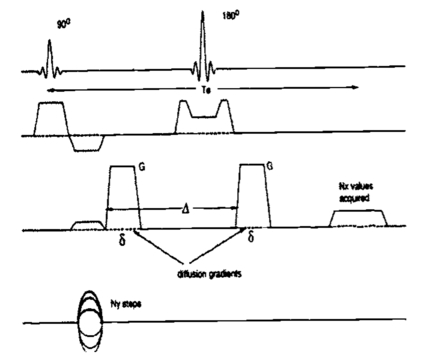

The use of diffusion imaging for non-invasive thermometry was proposed by Le Bihan in 1989²⁶. Delannoy et.al²⁸ demonstrated that diffusion imaging could used to measure temperature in a water-based gel phantom with a temperature resolution of ~0.5°C. Additionally, they accomplished this using a clinically relevant RF phased array heating device. The heating was gated so that the RF power was off during image acquisitions. In a highly controlled phantom experiment, Zhang et. al.²⁹ demonstrated that diffusion thermometry could give temperature resolution of 0.2°C in. 0.3cm³ voxels. Unfortunately, in vivo results were not as impressive. Diffusion imaging is exquisitely sensitive to object motion during the image acquisition. This is not a surprise since the objective is to measure the effects of molecular motion. Therefore a standard spin echo pulse sequence such as that in Fig. 13 is completely inadequate for in vivo applications.

Experiments in vivo using a single shot echo-planar imaging technique (see Fig. 13) were reported by McFall et. al.³⁰.

Fig. 14:

The echo-planar pulse sequence captures all of k-space in a single acquisition by using switching gradients with phase encoding “blips” between echoes.

These experiments were performed in the canine brain of normal animals. The animals were anaestitzed though out the heating procedure. A RF phased array was used to induce whole body hyperthermia. The imaging was cardiac gated to minimize pulsitile motion in the brain during the image acquisition. As whole body temperature approached 42°C, panting occurred and the dogs were paralyzed with atracurium to control breathing motion as well. Under these conditions, temperature resolution of 0.9°C in 0.89 cm³ was achieved. The measured sensitivity was with ε_a = 0.23eV.

More recently, improvements in hardware and software have produced higher and faster gradient fields and reductions in susceptibility artifacts. Thus, echo planar imaging has significantly improved as well. Using fast high-field gradients, MacFall et. al. examined the effect of tissue anisotropy on the temperature sensitivity of (ADC)³¹. This was done in vivo in the canine brain. The results show that although the ADC varies in the anisotropic white matter, the sensitivity to temperature remained the same (~2.5%/°C). To date there has not been a report of using the ADC technique in a clinical therapy application.